Designing Ann For Practical Application
Lab report AI: Designing ANN for practical application
Hardware used: I7 core, 8GB RAM
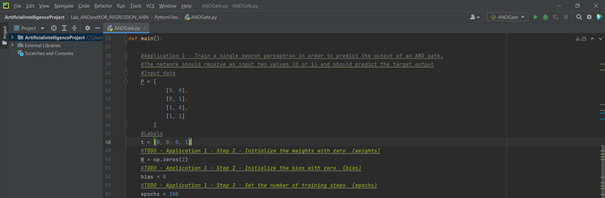
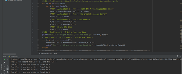
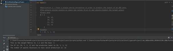
Application 1: AND GATE We designed an ANN with forward and back propagation to predict the AND GATE truth table. Below is the code to set up the correct weights and to compare the predicted label and the Ground Truth.
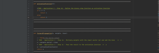
The forward propagation function, which return the predicted label for an input given the weight matrix and the bias, is defined as follow :
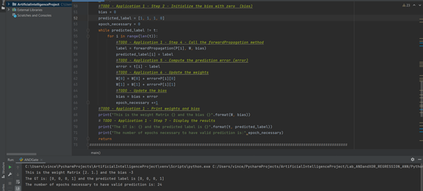
Exercise 1 : Number of epochs to obtain valid predictions To calculate this number we change the first for loop into a while loop that compares the predicted label and the Ground Truth. We add a counter to track the number of epochs. In the end, we need 24 eopchs to have valid predictions.
Exercise 2: Prediction for OR GATE To perform the prediction for the OR GATE, we just change the label vector as follow. We need 16 epochs to have the right predictions.
Exercise 3: Sigmoid activation function We define the sigmoid function as follow:

In the forward propagation function, we change the activation function for this one. The sigmoid function only returns value between 0 and 1 so it will never have the exact result.

The step unit function can return 0 and 1 which ensure that we will have convergence.

Application 2: XOR GATE For this application, we designed a simple 2-layer ANN, using 2 neurons in the first layer and 1 in the second. As in the previous application, we initialize the weights randomly and then perform both the back and forward propagation. We use here a sigmoid activation function.
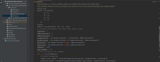
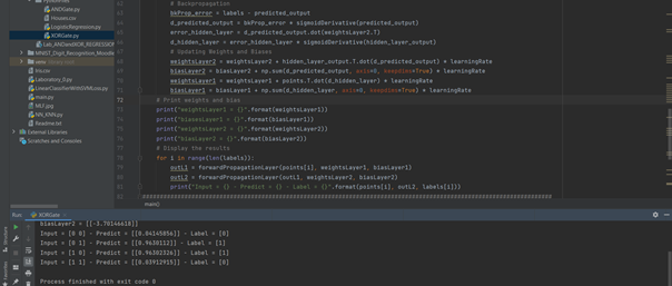
Exercise 4: Minimum number of epochs to have an error below 0.01 As before, we change the for loop into a while loop to have this number. We use a condition over the error of prediction and we implement a counter.
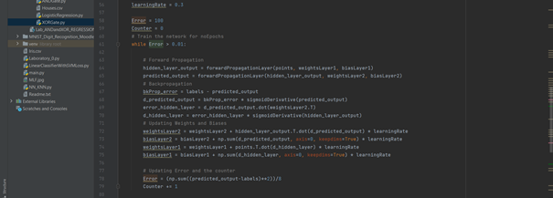
In the end, we need between 1400 and 3000 epochs to have an error inferior to 0.01. This number fluctuates because we randomly set the initial weights and bias. Sometimes, the algortihm does not converge at all.



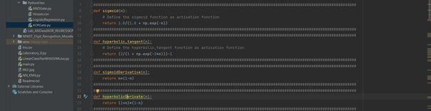
Exercise 5: Hyperbolic tangent as activation function We define the hyperbolic tangent function and its derivate. We change the activation function in the main.
Here are different results that we can get:



We can observe that the number of epochs has greatly decreased and is between 150 and 200. The predicted value also seems closer to the GT when it is close to 0 and seem a bit less accurate when it is close to 1.
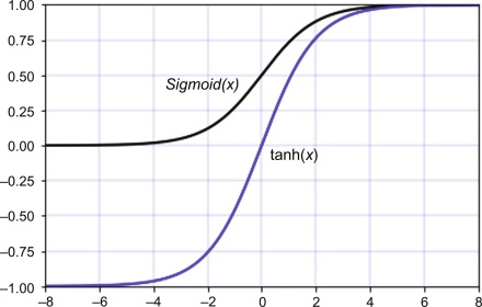
This may be explained by the fact tanh functions has output values between [-1,1] which means the function is symmetric and that the inputs will produce outputs centred around its mean = 0.
Exercise 6 : Number of trainable parameters The number of trainable parameters can be calculated as follow : 4 parameters for W1, 2 parameters for W2, 2 parameter for B1 and 1 parameter for B2. So in total, we have 9 parameters to train. The ANN performances are influenced by the initialization of the variables as mentionned in Exercice 4 and 5.
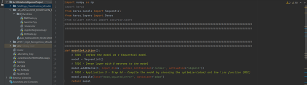
Exercise 7 : ANN architecture with Tensorflow We write the python script for the AND GATE with tensorflow as follow. We use only one layer with 1 neuron for this one as in the previous application.
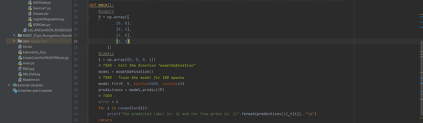
We use 3000 epochs considering the previous results of Exercice 4. We obtained the following results :

For the XOR GATE, we change the labels and add a layer as follow :


We have the following results :

For the 2 scripts, the results seem to close to the right label. We would need more epochs to have a better result.
Application 3: Regression House Price Market We use an ANN designed with Tensorfflow in this application to make a regression on the house price market given some inputs. We used a 2-layer ANN.

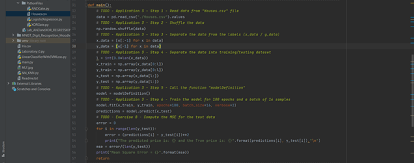
Here are some of the predicted prices and the corresponding true prices.
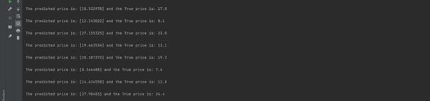
Exercise 8 : Mean square error We set up the MSE and run the algortihm a few times :





On average, we have an error of 0.116 thousand of dollars.
Exercise 9: Different values of MSE Before training the ANN, we shuffle the data which changes the training set each time. Some of them may output a better training model than others.
Exercise 10: MSE with 1 additional layer We add a layer in the model as follow :
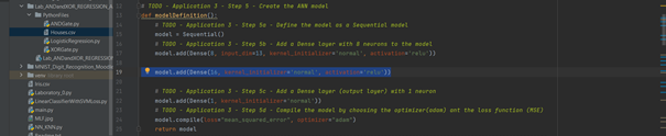



The MSE seem to be a bit better. On average, we have an error of 0.090 thousand of dollars. Having a an additional layer seem to improve a bit the predictions but it is more costly.
Exercise 11: Prediction of Nitric oxides concentration To predict this, we just change the input and output labels as follow. The old ones are:

And the new ones are :




The average MSE is 4.8e-05 parts per 10 million.